
In this paper we describe the technical underpinnings of FeatureBase, an analytical DBMS built around a bitmap-based data format. We'll start by defining some of the desirable performance characteristics of an analytical system so that we can show how those goals can be achieved in a bitmap-based system. We will describe how arbitrary data sets can be represented using bitmaps, including how high cardinality strings, integer, decimal, and timestamp columns are handled.
We will also discuss the (surprisingly few!) types of data which are not easily amenable to being represented as bitmaps and make a case as to why this isn't particularly important for analytics. Next, we'll walk through some surprising ways that typically complex schemas get simple representations, and why this is useful as well as how foreign key references are implemented.
We will describe the compression and storage techniques that allow FeatureBase to handle a wide variety of data, ingest, and query workloads while maintaining consistency and integrity of the stored data. We'll go over the general architecture for data ingestion, sharding, and parallel query execution. We'll conclude with a discussion of why we believe this type of system is uniquely positioned to serve the next generation of analytics workloads that go well beyond traditional business intelligence and decision support.
It's important to carefully define some terms up front. All of these words have generic meanings, but here we'll give more precise definitions in the context of characterizing and comparing analytical systems.
Latency: Specifically the latency of queries. How much time elapses between when a query is sent to a system and when the results return to the client. This is typically on the order of milliseconds to seconds, but some analytical queries can run for minutes, hours, or even days depending on the size of the data set and the hardware and software processing the query.
Freshness: This is like latency, but for data ingestion rather than querying. How much time elapses from when a data point is "sensed" by the system, until that data point will affect the results of a query? This can range from milliseconds to days depending on the data pipeline feeding the system.
Throughput: How much data can you ingest per unit time? Again this is specific to ingest, often there is a tradeoff between both latency and freshness, and throughput. A system that makes high-throughput ingest easy often has worse freshness, worse query latency, or both.
Concurrency: This is like throughput, but for queries. How many concurrent users can be running queries, and how much do they slow each other down? How much "analysis per second" can you do?
While FeatureBase uses a bitmap-based data format rather than a bitmap index, the principles are the same. The major difference is that, while the word "index" implies an auxiliary structure which is used to help speed up data access, FeatureBase uses the bitmap representation as its primary data storage.
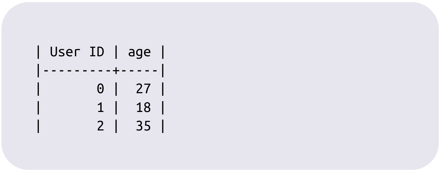
Bitmap indexes have been around since at least 1985, though implementations and usage have continued to evolve with significant improvements even during the last decade. To understand FeatureBase, it's important to have a solid mental model of a bitmap index. Given the following example table of people with their favorite ice cream, age, and hobbies:
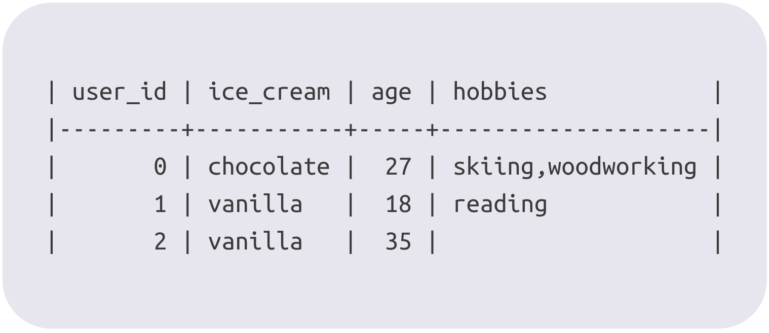
A bitmap index would be created on each column separately. In this way, a bitmap index is a form of columnar storage. The ice_cream column represented as a bitmap index would look as follows:
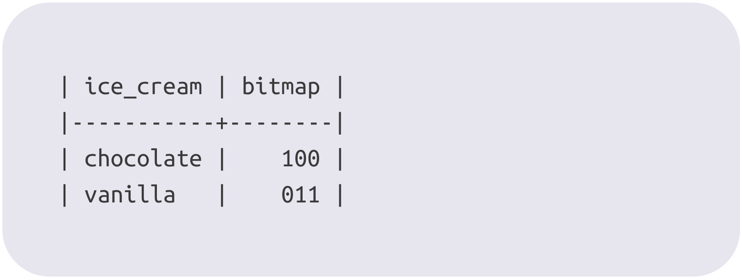
The two distinct values from the column ("chocolate" and "vanilla") are extracted, and a bitmap is created for each. The first "1" in the chocolate bitmap means that user_id 0 likes chocolate, while the two zeros mean that user_ids 1 and 2 do not like chocolate. Note that a bitmap index requires that each record corresponds to a position in the bitmap, and so each record must have, or be internally assigned a positive integer ID.
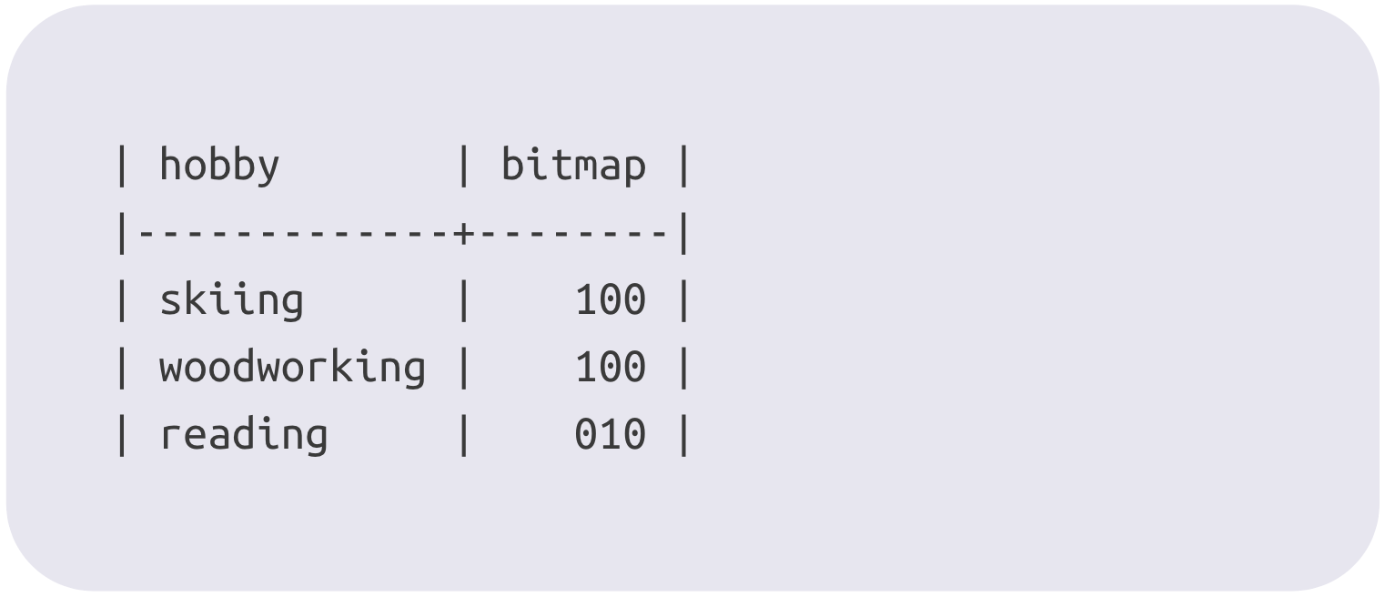
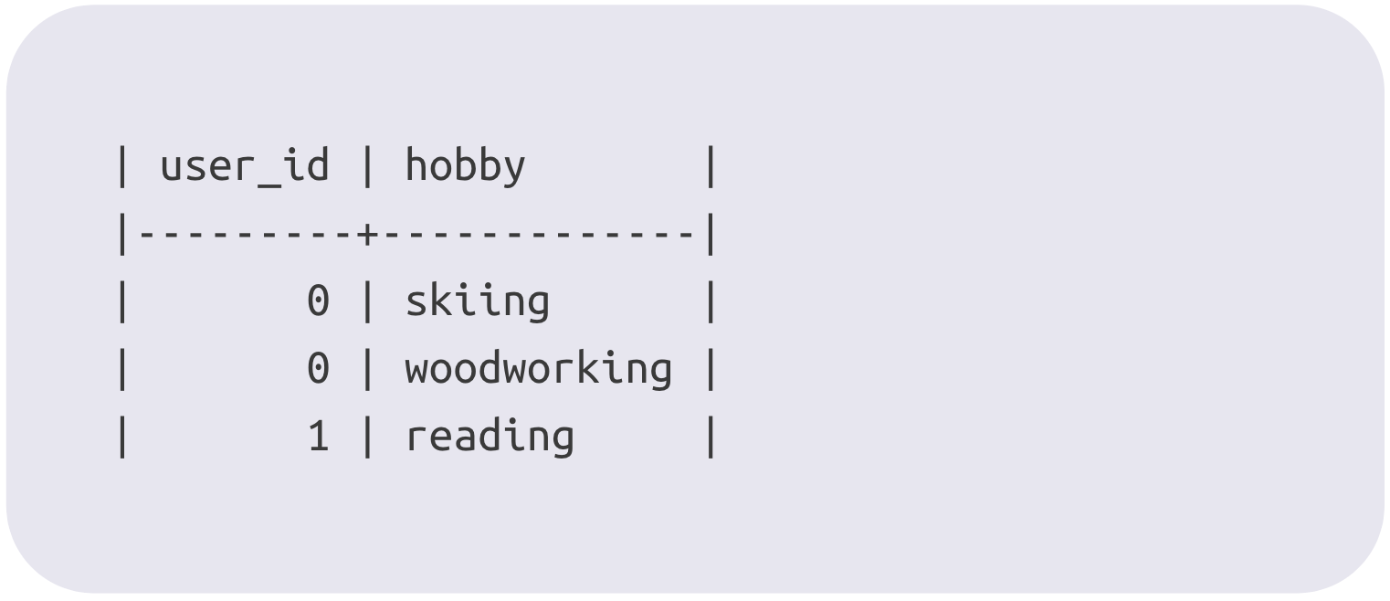
So, each bitmap for each distinct value in a column has a position which is reserved for each record in the table. The first position in the "vanilla" bitmap also corresponds to user_id 0, and is therefore set to 0 since user_id 0 likes chocolate and not vanilla. This leads to perhaps the most subtly powerful aspect of a bitmap index: any record can naturally have multiple values for a given column. To see this in action, here is the "hobbies" column represented as a bitmap index:
The implications of this will be discussed in depth later on.
The immediate benefit of a bitmap index is that it makes many queries much faster. Particularly, WHERE clauses, which are boolean combinations of categorical attributes, tend to be orders of magnitude faster if a bitmap index is used. For example, finding all chocolate-lovers who have a woodworking, but not a skiing hobby. This would result in the logical AND operation on the chocolate bitmap, the woodworking bitmap, and the inversion of the skiing bitmap. All of these operations can be done very efficiently on CPUs, and they do the absolute minimum amount of I/O because they only read the bitmaps related to the particular values which are of interest.
The structure of a bitmap index is inherently columnar, but as our example shows, actually goes further than that. Bitmap indexes have the unique capability of being able to access all data about a particular *value* within a column sequentially without having to scan over data about other values in the same column.
Bitmap indexes also allow the set of distinct values within a column to be stored separately from the data describing which records have which value(s) (i.e. the bitmap data). This is important because for categorical data, the set of distinct values tends to grow far slower than the number of records. Being able to access and analyze the set of values separately can be a great performance improvement for some queries, and the underlying storage can be better optimized for the particular use case.
The first objection to bitmap indexes is that they take up too much space. If there are 1M records in our table, then for a traditional representation we'd expect the ice_cream column to take 1M times 8 bytes assuming only two possible values and a roughly even split between vanilla and chocolate. So that's 8 megabytes to store the ice_cream column. In an uncompressed bitmap index, there are two bitmaps which are 1M bits long, plus the tiny overhead of storing the strings "chocolate" and "vanilla" each once.
That's only 2M bits or 1/4 of a megabyte. Not bad! However, the size of an uncompressed bitmap index scales with the cardinality of the field, not just the number of records in the field. If there are 10,000 possible hobbies, we could expect a normal database representation to maybe take up 20-30MB, whereas a bitmap representation would use 1.25GB! This is where bitmap compression comes into play.
A variety of schemes for compressing bitmaps have been proposed since the original bitmap index, but within the last decade, Roaring Bitmaps have risen to the top as the preferred way to compress and operate on bitmap indexes. Roaring splits every bitmap into containers that are 65,536 bits wide, and then chooses 1 of 3 encoding types for that container based on which will give the best compression. The three types are array, bitmap, and run. Arrays are for sparse containers that have few bits set; an array of 16 bit integers is kept which tells which of the 65,536 possible bits in the container are set. Bitmap containers are uncompressed and always take up 8KB (65,536 bits). Run containers are run-length encoded and can efficiently represent containers where most or all of the bits are set.
The key thing about Roaring though is not the compression types, but the fact that every bitwise operation (AND, OR, XOR, DIFFERENCE, NOT, etc.) is defined on every possible pair of encodings. This means that there's no decode-operate-encode, all operations take place on the data in the format it's already in. This means that any compression benefits double as performance benefits as, if you're interacting with array and run containers, you can often skip over large sections of containers in just a few processor instructions where no bit or all bits are set.
Having grasped the basics of bitmap indexes and the benefits of modern compression schemes, it's time to discuss some areas where bitmaps are not typically used, but are critical for an analytical system to support. These systems often need to store and analyze timestamps, costs, values from sensors, and other numeric data that can vary widely and rarely has repeated values.
The most common approach with a bitmap index would be to "bucketize" the data into a manageable number of categories so that they can be easily stored in bitmaps. This of course has the obvious issue of losing both query flexibility, and precise information about the exact value of each data point. If possible, it is best to store exact values and support queries over arbitrary ranges rather than fixed buckets.
Given all this, for numeric data a technique called bit-sliced indexing is used which enables encoding arbitrary 64 bit numbers without incurring the overhead of having a separate bitmap for each unique value. Even allowing for compression, a bitmap-per-value would be very inefficient for something like "home sale prices", and a query like "how many homes sold for over $1M would have to union all the bitmaps for values over $1M of which there could be many thousands.
To briefly describe bit-sliced indexing, there is a bitmap for each possible binary digit of the values in a column, and when a value is added to a record, a bit is set in each of the digit bitmaps for each digit in that value which is 1 in its binary representation. As an example, if we had a column whose values were all between 0 and 7, and a new record was added that had a value of 5, we'd set bits in the 1st and 3rd bitmaps of this column.
For the age column of our original table, the BSI representation would look like (the 2^<digit> column is just a convenience to see what the decimal value of each digit is):
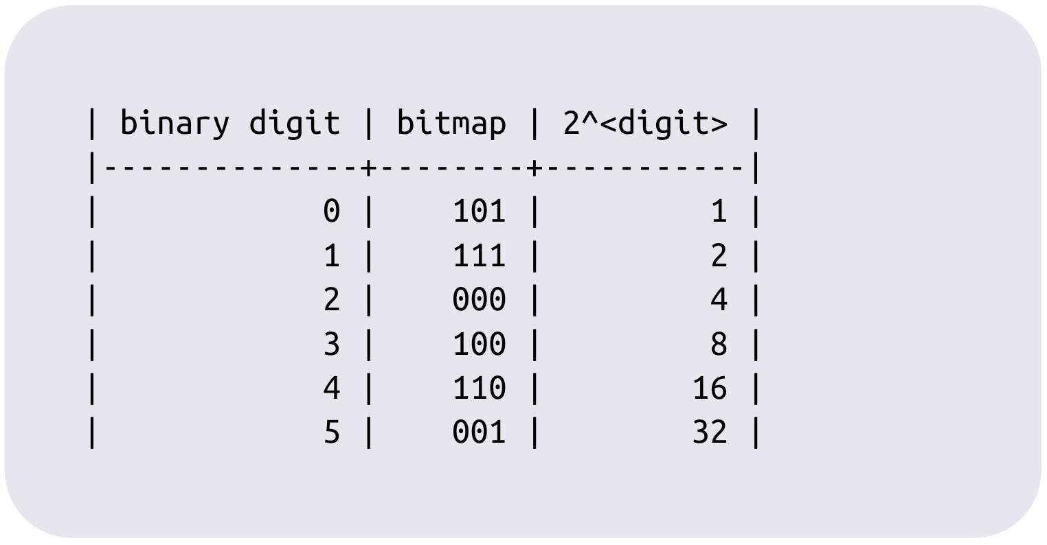
Here are the original values:
If you run down each column of bits in the bitmap column, and add up the values from 2^<digit> wherever there is a 1 in the bitmap column, you'll get the age values from the original table. The full mechanics of making arbitrary range queries over this data are covered in depth in the original papers which introduced BSI, but consider a simple example. How would we count the number of people with age greater than 15? It would simply be the union of the bitmaps for binary digits 4 and 5 (and any higher digits that happened to exist in the data), and then counting the number of set bits in the resulting bitmap.
What BSI means is that we can represent any number in the 64 bit range (~10^19) using only 64 bitmaps. It turns out that queries over arbitrary ranges of the values can be completed via boolean combinations of the underlying bitmaps. This means that integer, timestamp, and fixed-point decimals can all be handled efficiently by a bitmap storage engine. A bit-sliced implementation of floating point may also be possible but is an area of future research.
We've discussed how bitmaps are used to encode a variety of different types of data, including fairly high cardinality categorical data, and arbitrary numerical data, but there are some things best left out of a bitmap index.
While high cardinality isn't as much of an issue one might expect, at some point the use of bitmaps doesn't make sense any more. Consider the humble email address. Emails don't necessarily have a 1:1 mapping with people, but they are relatively rarely shared between many people. Are you particularly interested in questions like "how many people have this email address?", or "what email addresses are most common in my data set?". If those sound a bit silly, it's because they are! You might be interested in the most common email domains, but that's a different feature that would be useful to store. The reason to store emails or phone numbers, or other identifying/contact type information is so that once you've identified an interesting set of records through analysis, you can actually *do* something with them.
For this type of information it's generally sufficient for it to be stored separately, so it isn't eating I/O from your analytics workloads, but is available for simple key/value lookup when you need it.
Note: separately need not mean "outside the database", just not intermingled with the data that is useful for analysis.
All of these things require some amount of pre-processing to be very useful in a structured relational-type database. For images and videos, you can easily extract metadata like creation date, location, equipment specs, etc. You can even do more advanced things like storing the average color of an image or its overall variability etc. Similarly, for text blobs (and genomes) you could extract n-grams for analysis and a variety of other creative things, but serializing the thing itself into a bitmap probably isn't useful. You want to store features in bitmaps. That's why it's called FeatureBase ;).
This isn't supported today, but there's reason to think that an extension of bit-sliced indexing could support it. We're also experimenting with a method to store data in more of a normal columnar fashion for some columns (e.g. floating point, or mostly unique string identifiers). Stay tuned :)
As discussed above, for typical categorical data (e.g. ice cream flavor, hobbies) every possible value of a field has an associated bitmap that tells you which records have that value. This leads to a very interesting and useful characteristic of a bitmap-based storage system: any record can have many values for one field with essentially no overhead. Observe:
The first user has both skiing and woodworking as hobbies, the second user has just reading, and the third user has no hobbies at all. In FeatureBase, these are called 'set' fields as each record can have a set of values. Most databases would represent this with a separate table that looked like:
Having a separate table is very flexible, you can add new columns and have very rich query capabilities across them and the original table, however the tradeoff is query speed and storage efficiency—packing all this info into a single column that's in the same table as the rest of the data you’re querying brings massive performance benefits.
There's one more trick that FeatureBase does with bitmap-based storage to give you some of the flexibility of having a separate table while keeping the benefits of having the information in the same column. It's called "time quantums", and it essentially gives you the ability to add one more piece of information to every set bit in the field. Let's start with an example: how would you go about storing each person's hobbies, and which month they started getting into each hobby? If you have the data in a separate table, you just add a column like so:
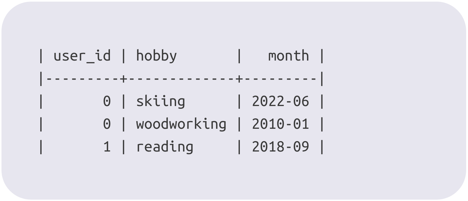
In FeatureBase, you can attach this information directly to the existing "hobbies" set field within a table by using a time quantum. This will allow you to answer queries like "how many people got into reading between 2009 and 2019?", "did more people get into woodworking in the Summer of 2009 or 2010?". The way this is accomplished is through something called "views" — FeatureBase will actually store a separate bitmap for each month present in the data, and when you query across a time range it will union several bitmaps together to get an answer.
One must be careful to find the right granularity to use—if the data is too sparse at the chosen granularity, it will become memory intensive and queries will be slower, but if the granularity is too coarse one may not be able to answer all the questions they want to ask. Time quantums are mostly suitable when you have a well understood workload and need the best query performance possible, but they are a powerful tool in this scenario and aren't offered by any other database.
The good news is, if time quantums don't fit your use case, a traditional data model is still an option. FeatureBase supports foreign key relationships between tables, so one can use the values from a column of one table as a filter on another table. Recall that early on we discussed how every record and value in FeatureBase has an integer ID associated with it. The record ID of one table can be stored in a field of another table. This can be either a BSI field, or a normal set field. FeatureBase can find all the distinct values of a particular field for a subset of its records and return them as a bitmap—that bitmap can then be treated as a special temporary value of another table and used to filter it.
Having covered at a high level how data is stored in bitmaps, it's time to dive into the nitty gritty of what happens if you actually try to build a DBMS with a bitmap storage engine, and particularly what happens at scale.
In order to distribute data across multiple machines, one must decide on a sharding strategy. In FeatureBase, sharding controls both how data is distributed, and what data can be operated on concurrently within a single query. Recall that the bitmap data is stored separately from the key data (the distinct values of a field that map to bitmaps)—our discussion here will focus primarily on the bitmap data as that's where the bulk of the query computation tends to happen, and it is the part that is most novel in FeatureBase.
The bitmap data in FeatureBase is sharded by records. By default there are 2^20 (about 1M) records in a shard. All the bitmap data for a shard, for all the fields in a table is stored in an embedded RBF database. RBF stands for Roaring B-tree Format which we'll discuss in more depth in the next section. For now, know that it is an embedded storage engine specifically designed for bitmaps that supports a single writer but many concurrent readers using MVCC and provides ACID guarantees.
For many typical analytical queries, large portions of the query processing can be done in parallel across all shards. The query is sent to every node containing relevant shards, and then that node launches a task for each shard that needs to be processed. Read-only memory within RBF can be shared by many queries and swapped out if it isn't in use, the only heap allocations needed are to hold results which are reduced locally for all shards within a node, and then whichever node is coordinating the query aggregates results from all the other nodes.
For the key data, there are actually two distinct categories in FeatureBase, the one that we've talked about already is the column keys. The column keys for a particular column are essentially all the distinct values of that column mapped to numbers, and the numbers will locate the bitmap that goes with that value in each RBF store. While in theory, each shard might have a completely distinct set of values for each field, that wouldn't be very useful for analytics (like the email address example above), and in practice there's a lot of overlap in the set of column values that each shard has. Because of this, the value-to-bitmap mapping is stored just once* rather than being stored separately for each shard.
The other category of key data is the record keys. Recall that every record in a FeatureBase table maps to an integer value which is an index into each of the bitmaps. Sometimes this mapping is direct in that the record already has an integer identifier which is suitable for this purpose, and sometimes the table is "keyed" meaning that the record identifier is treated as a string and a mapping is created to its integer ID. Because these mappings are tied directly to records, they are generally kept adjacent to the shards they belong to (though this is not a requirement).
Query processing in FeatureBase goes through a translation phase where all string keys (both column and record) are translated to IDs, then the query is processed, then any integer IDs in the results are translated back to keys as necessary.
For each shard's bitmap storage, we use a custom embedded storage engine called RBF (Roaring B-Tree Format). As the name implies, this format stores Roaring Bitmaps in a B-Tree structure.
FeatureBase has a fairly demanding set of requirements for its storage engine in that reads, writes, and, crucially, updates need to be really fast, and of course the storage must be durable and support atomic writes without any consistency or integrity issues. The one saving grace is that for analytical workloads it's not generally important to support very granular transactions at high throughput—small batches of records can be aggregated and written all at once.
RBF manages to achieve totally non-blocking concurrent reads - reads are never blocked either on other reads or on writes. Due to its write-ahead log and snapshotting capabilities, it also supports high throughput writes from a single writer at a time, and is engineered for ACID compliance.
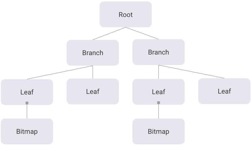
RBF uses 8KB pages, the initial pages are used for metadata and root pages (a single RBF database can contain multiple B-Trees within it, and therefore multiple roots). Each root page points to branch pages which point to leaf pages that contain actual bitmap data. Each bitmap within a shard is a fixed width of 2^20 records, but can take up wildly varying amounts of space based on the actual data contained within. Roaring Bitmaps are composed of containers each of which is 2^16 (65,536) bits wide, so one value for a shard is 16 containers wide.
The maximum size of a container is when it is represented as a raw bitmap and takes up exactly 8KB (65536 bits) of data which fits neatly into an RBF page. Each container does have header information though, so bitmap containers are actually stored as children of leaf nodes and only their headers are contained within the leaf pages. Other containers' headers and data are contained entirely within leaf pages. When containers are significantly smaller than 8KB which happens frequently with Roaring's run-length and array encodings, multiple can be packed into a single page.
The RBF database is composed of two memory-mapped files, one is the database itself, and the other is the write-ahead log or WAL. When a write comes in to RBF at least one entire page is always written. Any changes to pages are made in memory, then the changed pages are appended to the WAL. Once those changes have been fsynced to disk, new reads will use the versions in the WAL rather than the versions in the main file. Periodically, if there are no transactions going on, or if the WAL is too large, the new pages will be written back to the main database in a process called checkpointing, the WAL will then be truncated and all reads will come solely from the main database file until new writes occur.
Data ingestion for analytics purposes is a historically fraught endeavor. While analytics read workloads benefit immensely from columnar formats and sophisticated indexing schemes, these things cause write performance to suffer. Columnar on its own means that a write of a single record incurs a separate disk access for each column, as they're stored in different places, and additional indexes incur further writes.
Even worse though, many storage formats and indexing schemes are not easily updated in-place, and often large chunks of data must be overwritten to incorporate small changes. Because of these challenges, many analytics solutions rely on batch ingests sometimes running overnight to prepare data sets for analysis.
Bitmap indexes, and FeatureBase by extension, are not immune to these challenges. FeatureBase leverages a wide variety of techniques to achieve high throughput and sufficient freshness on incoming data. To illustrate these techniques, here is an example scenario where FeatureBase is ingesting data from a Kafka:

The first optimization is to add data to Kafka such that its partition key is the same as FeatureBase uses to partition data internally which is a fairly straightforward hash. This means that each of the concurrent ingester processes will read data that is bound for a smaller subset of shards within FeatureBase rather than being spread randomly across many shards.
Secondly, the ingester processes are separate from FeatureBase and have the sole job of reading data from Kafka and putting it into a format that FeatureBase can accept most efficiently. Having separate ingester processes allows them to be scaled independently of FeatureBase, and the hardware can be optimized for that particular workload.
Because the key and bitmap data is separate in FeatureBase, the ingesters split the process of ingestion into "key translation" and "bitmap ingestion" stages. An ingester reads a batch of records, finds all the keys that need to be translated for that batch, and sends a key translation request to FeatureBase. Once it has the integer IDs that correspond to all the keys in the batch, it can build bitmaps of all the incoming data locally, and then send the compressed bitmaps to FeatureBase.
Often, the ingester is able to cache many of the keys, particularly the column keys since the domains of each column are often fairly constrained and don't get new values frequently. This reduces network traffic, and improves overall ingest performance as only compressed bitmaps representing the new relationships in the data need to be handled by FeatureBase.
Note: the configurable batch size on ingesters usually represents a tradeoff between throughput and freshness as we defined earlier. Larger batches offer greater throughput at the expense of freshness. For most use cases the desirable throughput is achieved with a freshness ranging from seconds to a few minutes.
Once bitmap data hits FeatureBase, the incoming bits are unioned with and/or differenced from the existing data depending on whether data is being added, updated, or deleted. FeatureBase is somewhat unique in that it manages to support high throughput updates rather than just appends. Any pages which have changes after all incoming bits are applied in memory are written to the write ahead log. All writes happen atomically within a shard, so partial updates are never seen by concurrent reads.
Updates in particular can incur a lot of disk I/O writing many pages, so for update-heavy workloads FeatureBase is often configured with some combination of very fast disks, arrays of disks, and more nodes to provide the necessary I/O bandwidth. We have seen implementations achieve >1 million updates per second using these optimizations.
We started off by defining terms that define desirable performance characteristics of an analytical system. These are Latency, Throughput, Freshness, and Concurrency. To summarize them briefly, the ideal analytical system should support very fast queries that return information on your newest data, and should be able to handle as much incoming ingest and query workload as necessary.
Most systems make sacrifices in at least one of these areas in order to achieve acceptable levels of performance in the others. The areas which are most commonly left lacking are Freshness and Latency. What this means is that most organizations don't view their analytics capability as a real-time or interactive component of their operations. Either they're operating on data which is hours to days old, or their queries and reports take hours to build.
Being able to operate on the latest data interactively is not just an incremental improvement, it opens up new use cases and elevates analytics from a decision support system, to potentially a whole new line of business. FeatureBase makes this happen by rethinking analytics technology from the storage layer up.
Latency: FeatureBase achieves extremely low latency queries by storing data in a form that is both more compact *and* more granularly accessible for analytics. This means dramatically less I/O per query, *and* data is stored in a form that's usually more efficient to perform computations on.
Freshness: FeatureBase provides analytics on fresh data by optimizing every stage of the ingest path and storage engine to allow small batches of data to be ingested quickly without impacting ongoing queries.
Throughput: FeatureBase delivers high throughput ingest performance by allowing ingestion to scale independently of query processing, and optimally sorting and formatting incoming data before it ever hits the database.
Concurrency: More efficient queries and storage on a more scalable system means you can handle more concurrent queries with the same amount of hardware, and add more hardware when the workload demands it.
*Stored once *notionally*. In some cases it is replicated for performance/durability reasons. The point is, it isn't necessarily stored alongside each shard which is a significant departure from your typical database.


